


What if you have two data
sources, such as flat files or table data, and have to merge or join them
together? If there is a common attribute, such as customer ID, the solution
should be pretty obvious: join the related attribute, and in this example, the
customer ID suffices. What if the sources have nothing in common? The only
requirement is that a record in source 1 gets matched up to a record in source
2. Further, it doesn’t matter *which* particular record gets matched to another,
what does matter is that every record in one source gets tagged with a record
from the other source.
The above problem can be
described as having to join disparate or seemingly unrelated data. In a prior
article, I covered the use of ROWNUM to create an association between
uncorrelated data. The essence of this join method is take advantage of an
Oracle-provided pseudo column to create the linkage. The query below can be used
as part of a CREATE TABLE AS SELECT statement or as an insert into an already
existing target table based on the joined conditions.
SELECT * FROM
(SELECT <COLUMNS OF INTEREST>, ROWNUM AS rownum_a
FROM TABLE_A
<USING A WHERE CLAUSE IF NEED BE>) ALIAS_A,
(SELECT <COLUMNS OF INTEREST>, ROWNUM AS rownum_b
FROM TABLE_B
<USING A WHERE CLAUSE IF NEED BE>) ALIAS_B
WHERE ALIAS_A.rownum_a = ALIAS_B.rownum_b;
What is a potential drawback
to this method, assuming the number of records to be joined is large (as in
millions)? Well, when is the row number “calculated” for a record? We don’t
have real control over the order in which rows are returned in a query, and
Oracle has no idea of a record’s row number until we execute a query. In other
words, ROWNUM is established after the fact. If you’re selecting millions of
rows from two places, you’re going to pay for the time it takes for Oracle to
assign (for the purposes of your query, but not forever) a row number for each
and every record.
Let’s trace a session that
joins two one-million tables together. In this first example, the sources are
already populated with one million records. Table A ranges from 1 to 1,000,000
and Table B ranges from 1,000,001 to 2,000,000 (i.e., add a million to the
value in the first table). If the join is perfect in the sense of maintaining
row order, then the ordered pairs will look like so:
|
1 |
1,000,001 |
|
2 |
1,000,002 |
|
3 |
1,000,003 |
|
4 |
1,000,004 |
|
5 |
1,000,005 |
|
Etc |
Etc |
What we find when viewing
the data (via Toad) is that Oracle does not perform a perfect ordering, and is
far from it.
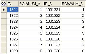
The ROWNUM_A and B values
will match from record to record because that is what we matched/joined upon.
Note how record 1321 (and 1001321) were tagged with a ROWNUM of 1. All we can
deduce about that is that Oracle filled an empty block in the same manner
between the tables. This should convince you once and for all (if you didn’t
already know) that the ROWNUM pseudo column has no meaning or relevance to the
actual order of records in a table.
A trace taken of the create
table statement, after being TKPROF’d, yields the following:
CREATE TABLE TABLE_ROWNUM AS
SELECT * FROM
(SELECT ID, ROWNUM AS rownum_a
 FROM TABLE_A)
 ALIAS_A,
(SELECT ID AS id_b, ROWNUM AS rownum_b
 FROM TABLE_B)
 ALIAS_B
WHERE ALIAS_A.rownum_a = ALIAS_B.rownum_b
call     count       cpu    elapsed       disk      query    current        rows
------- ------  -------- ---------- ---------- ---------- ----------  ----------
Parse        1      0.01       0.00          0          0          0           0
Execute      1      4.41       5.63       1770      12324       5239     1000000
Fetch        0      0.00       0.00          0          0          0           0
------- ------  -------- ---------- ---------- ---------- ----------  ----------
total        2      4.42       5.64       1770      12324       5239     1000000
We know for a fact that each
table has one million rows in them. After analyzing the tables, the value for
NUM_ROWS shows 1,034,591. Be careful about relying on values surfaced through a
third party tool (including selecting NUM_ROWS from USER_TABLES) when compared
to what Oracle itself will report via a straight count. Why would there be a
discrepancy here? Is the analyze statement based on a sample or estimate of the
data, or upon an examination of each and every record?
Now, on to an alternate
means of joining the data. Instead of a pseudo column, let’s use a real one,
and a natural choice is to create (in a sense) a surrogate key based on a sequence.
The setup is to add a column named SEQ to each table and update it based on a
sequence, where each update uses the same starting value and same increment.
One of the tables’ update is shown below.
SQL> create sequence tab_b;
Sequence created.
Elapsed: 00:00:00.05
SQL> update table_b set seq = tab_b.nextval;
1000000 rows updated.
Elapsed: 00:05:00.05
One thing should immediately
stand out: the time it took to create the join key was just over five minutes,
or over 13 times as much time for the setup as the ROWNUM method took, and that
is for just one of the two tables (the first table also took five minutes to
update). The addition or creation of the join key needs to be done, if at all
possible, concurrently with the creation of the table proper. Otherwise, what’s
the point of spending more time than what can be done via ROWNUM?
Under the new setup, how
does the merge perform?
CREATE TABLE TABLE_SEQ AS
SELECT * FROM
(SELECT ID, SEQ AS seq_a
 FROM TABLE_A)
 ALIAS_A,
(SELECT ID AS id_b, SEQ AS seq_b
 FROM TABLE_B)
 ALIAS_B
WHERE ALIAS_A.seq_a = ALIAS_B.seq_b
call     count       cpu    elapsed       disk      query    current        rows
------- ------  -------- ---------- ---------- ---------- ----------  ----------
Parse        1      0.00       0.06          0          0          0           0
Execute      1     10.64      24.43      12186      12370       5677     1000000
Fetch        0      0.00       0.00          0          0          0           0
------- ------  -------- ---------- ---------- ---------- ----------  ----------
total        2     10.64      24.49      12186      12370       5677     1000000
Interestingly, now that the
data isn’t so disparate, the performance is slightly worse. What do the explain
plans show? For the original test using ROWNUM, we have:
PLAN_TABLE_OUTPUT
-------------------------------------------------------------------------------------------------
Plan hash value: 1354216904
-----------------------------------------------------------------------------------------------
| Id  | Operation              | Name         | Rows  | Bytes |TempSpc| Cost (%CPU)| Time     |
-----------------------------------------------------------------------------------------------
|   0 | CREATE TABLE STATEMENT |              |    10G|   496G|       |    15M  (2)| 50:40:43 |
|   1 |  LOAD AS SELECT        | TABLE_ROWNUM |       |       |       |            |          |
|*  2 |   HASH JOIN            |              |    10G|   496G|    36M|   186K (97)| 00:37:19 |
|   3 |    VIEW                |              |  1009K|    25M|       |  1597  (10)| 00:00:20 |
|   4 |     COUNT              |              |       |       |       |            |          |
|   5 |      TABLE ACCESS FULL | TABLE_B      |  1009K|  4930K|       |  1381  (11)| 00:00:17 |
|   6 |    VIEW                |              |  1016K|    25M|       |  1475  (10)| 00:00:18 |
|   7 |     COUNT              |              |       |       |       |            |          |
|   8 |      TABLE ACCESS FULL | TABLE_A      |  1016K|  3969K|       |  1285  (12)| 00:00:16 |
-----------------------------------------------------------------------------------------------
Predicate Information (identified by operation id):
---------------------------------------------------
   2 - access("ALIAS_A"."ROWNUM_A"="ALIAS_B"."ROWNUM_B")
The sequence-based join has
what appears to be a better plan.
PLAN_TABLE_OUTPUT
-------------------------------------------------------------------------------------------------
Plan hash value: 1354216904
-----------------------------------------------------------------------------------------------
| Id  | Operation              | Name         | Rows  | Bytes |TempSpc| Cost (%CPU)| Time     |
-----------------------------------------------------------------------------------------------
|   0 | CREATE TABLE STATEMENT |              |    10G|   496G|       |    15M  (2)| 50:40:43 |
|   1 |  LOAD AS SELECT        | TABLE_ROWNUM |       |       |       |            |          |
|*  2 |   HASH JOIN            |              |    10G|   496G|    36M|   186K (97)| 00:37:19 |
|   3 |    VIEW                |              |  1009K|    25M|       |  1597  (10)| 00:00:20 |
|   4 |     COUNT              |              |       |       |       |            |          |
|   5 |      TABLE ACCESS FULL | TABLE_B      |  1009K|  4930K|       |  1381  (11)| 00:00:17 |
|   6 |    VIEW                |              |  1016K|    25M|       |  1475  (10)| 00:00:18 |
|   7 |     COUNT              |              |       |       |       |            |          |
|   8 |      TABLE ACCESS FULL | TABLE_A      |  1016K|  3969K|       |  1285  (12)| 00:00:16 |
-----------------------------------------------------------------------------------------------
Predicate Information (identified by operation id):
---------------------------------------------------
   2 - access("ALIAS_A"."ROWNUM_A"="ALIAS_B"."ROWNUM_B")
Even though this is a
relatively small data set, you can see why cost in an execution plan can be
misleading. If the sequence-based table is dropped and re-created within the
same session, the time to create the table anew drops to just over two seconds.
At face value, the second round of creating the table appears to be much
faster, but what does that really prove?
All it proves is that with
blocks already read into cache, the reading of the blocks is going to be much
faster than reading from disk (which we already know to be true). The practical
implication is this: how many times do you need to create the table? It’s
usually a one time deal. If the original table is dropped and re-created, it’s
time to create is also substantially faster.
Leveling the playing field
by flushing the shared pool and buffer cache, the time comparisons are
(approximately) 14 seconds and 10 seconds in the ROWNUM and sequence cases. At
this point, it may seem like the cases are confused. Between runs, the
performance ranking switches. That may be the case, but don’t forget the cost
(in terms of time) it took to setup the sequence-based tables.
In Closing
At some point, most likely
data set, operating system and platform dependent (how many millions of rows,
RAM, I/O, etc.), it may be faster to add a common attribute between disparate
data sets before creating the merged table. For smaller sets of data, perhaps
something a bit above a million rows, I would venture to say that it will
always be faster to use ROWNUM than to add a join key, even if the actual
create table operation using the common key is faster. So, when is it (more)
appropriate to use ROWNUM? In cases when there is no common key and you don’t
care about the specific associations between tables, just that one does take
place. If you are working with related tables, based on a common attribute, and
the association has to be ordered, you definitely cannot rely upon ROWNUM to
maintain the ordered join between tables. It does matter that a specific row in
one table is matched with a specific row in the second table.